## # A tibble: 100 × 20
##         V1      V2     V3      V4      V5      V6      V7      V8     V9    V10
##      <dbl>   <dbl>  <dbl>   <dbl>   <dbl>   <dbl>   <dbl>   <dbl>  <dbl>  <dbl>
##  1  0.274  -0.0367  0.855  0.968   1.42    0.523   0.563   1.11    1.64   0.619
##  2  2.24   -0.546   0.234 -1.34    1.31    0.521  -0.610  -0.861  -0.270  0.230
##  3 -0.125  -0.607  -0.854 -0.149  -0.665   0.607   0.162  -0.863   0.604  1.19
##  4 -0.544   1.11   -0.104  1.02    0.700   1.66    0.490   0.0234  0.256 -0.127
##  5 -1.46   -0.274   0.112 -0.852   0.315   1.05    1.39    0.285   1.14   2.68
##  6  1.06   -0.754  -1.38   1.08    0.370   1.50   -0.360  -0.214   1.83   0.871
##  7  0.116  -0.966   0.274  0.0185 -0.210   0.544  -2.51    2.20    0.593 -1.09
##  8  0.390   0.400  -0.467  0.478   0.848   0.257  -0.0995  0.999  -0.193 -0.404
##  9  0.193   0.197  -1.24   1.91    0.115   0.452  -0.267  -0.273  -1.61  -0.326
## 10 -0.0964  1.18    2.55   0.956   0.0256 -0.0456 -0.659   0.0392  0.172  0.643
## # … with 90 more rows, and 10 more variables: V11 <dbl>, V12 <dbl>, V13 <dbl>,
## #   V14 <dbl>, V15 <dbl>, V16 <dbl>, V17 <dbl>, V18 <dbl>, V19 <dbl>, V20 <dbl>
## # A tibble: 100 × 1
##        V1
##     <dbl>
##  1 -1.27
##  2  1.84
##  3  0.459
##  4  0.564
##  5  1.87
##  6  0.528
##  7  2.43
##  8 -0.895
##  9 -0.206
## 10  3.11
## # … with 90 more rows
## Perform ridge regression with 10-fold CV
ridge1_cv <- cv.glmnet(x = x_cont, y = y_cont, type.measure = "mse",
                       lambda = exp(seq(-5,-1.5, length.out = 100)),
                       nfold = 10, alpha = 0) # alpha is the e-net mixing par
## Penalty vs CV MSE plot
plot(ridge1_cv)
abline(v = log(ridge1_cv$lambda.min))
## 21 x 1 sparse Matrix of class "dgCMatrix"
##                       s1
## (Intercept)  0.132825360
## V1           1.334864503
## V2           0.031514349
## V3           0.739492669
## V4           0.048358071
## V5          -0.881162824
## V6           0.611469081
## V7           0.123949760
## V8           0.386769953
## V9          -0.038636714
## V10          0.118120656
## V11          0.245469489
## V12         -0.067686451
## V13         -0.045130346
## V14         -1.121405223
## V15         -0.130593351
## V16         -0.042130893
## V17         -0.045664317
## V18          0.060068396
## V19         -0.003373719
## V20         -1.108136513
## Perform adaptive LASSO with 10-fold CV
alasso1_cv <- cv.glmnet(x = x_cont, y = y_cont,
                        type.measure = "mse",
                        nfold = 10,
                        alpha = 1,
                        penalty.factor = 1 / abs(best_ridge_coef),
                        keep = TRUE)
## Penalty vs CV MSE plot
plot(alasso1_cv)
## 21 x 1 sparse Matrix of class "dgCMatrix"
##                     s1
## (Intercept)  0.1252790
## V1           1.3872769
## V2           .
## V3           0.7552762
## V4           .
## V5          -0.8925767
## V6           0.5683429
## V7           .
## V8           0.3623266
## V9           .
## V10          .
## V11          0.1748004
## V12          .
## V13          .
## V14         -1.1146180
## V15          .
## V16          .
## V17          .
## V18          .
## V19          .
## V20         -1.1239692
library(VGAM)
plot(y = dlaplace(seq(-3,3, length.out = 1000), scale = 1),
     x = seq(-3,3, length.out = 1000), type = "l",
     main = "Laplace distribution", ylab = "density", xlab = "")
## stan_glm
##  family:       gaussian [identity]
##  formula:      y ~ .
##  observations: 100
##  predictors:   21
## ------
##             Median MAD_SD
## (Intercept)  0.1    0.1
## x.1          1.4    0.1
## x.2          0.0    0.1
## x.3          0.8    0.1
## x.4          0.1    0.1
## x.5         -0.9    0.1
## x.6          0.6    0.1
## x.7          0.1    0.1
## x.8          0.4    0.1
## x.9          0.0    0.1
## x.10         0.1    0.1
## x.11         0.3    0.1
## x.12        -0.1    0.1
## x.13        -0.1    0.1
## x.14        -1.2    0.1
## x.15        -0.1    0.1
## x.16        -0.1    0.1
## x.17        -0.1    0.1
## x.18         0.1    0.1
## x.19         0.0    0.1
## x.20        -1.1    0.1
##
## Auxiliary parameter(s):
##       Median MAD_SD
## sigma 1.0    0.1
##
## ------
## * For help interpreting the printed output see ?print.stanreg
## * For info on the priors used see ?prior_summary.stanreg
##  (Intercept)          x.1          x.2          x.3          x.4          x.5
##  0.110978758  1.383406675  0.023433696  0.767465639  0.066199186 -0.903181023
##          x.6          x.7          x.8          x.9         x.10         x.11
##  0.619143984  0.125173599  0.402498695 -0.038407595  0.134344297  0.252355538
##         x.12         x.13         x.14         x.15         x.16         x.17
## -0.070953063 -0.050532662 -1.165130179 -0.145895451 -0.054105129 -0.056000871
##         x.18         x.19         x.20
##  0.050886785 -0.004531585 -1.144454727
## stan_glm
##  family:       gaussian [identity]
##  formula:      y ~ .
##  observations: 100
##  predictors:   21
## ------
##             Median MAD_SD
## (Intercept) 0.7    0.3
## x.1         0.0    0.0
## x.2         0.0    0.0
## x.3         0.0    0.0
## x.4         0.0    0.0
## x.5         0.0    0.0
## x.6         0.0    0.0
## x.7         0.0    0.0
## x.8         0.0    0.0
## x.9         0.0    0.0
## x.10        0.0    0.0
## x.11        0.0    0.0
## x.12        0.0    0.0
## x.13        0.0    0.0
## x.14        0.0    0.0
## x.15        0.0    0.0
## x.16        0.0    0.0
## x.17        0.0    0.0
## x.18        0.0    0.0
## x.19        0.0    0.0
## x.20        0.0    0.0
##
## Auxiliary parameter(s):
##       Median MAD_SD
## sigma 2.9    0.2
##
## ------
## * For help interpreting the printed output see ?print.stanreg
## * For info on the priors used see ?prior_summary.stanreg
##   (Intercept)           x.1           x.2           x.3           x.4
##  6.525370e-01  2.349271e-03  5.342229e-04  9.873049e-04 -8.862767e-06
##           x.5           x.6           x.7           x.8           x.9
## -1.045235e-03  1.267102e-03  1.813045e-04  5.819743e-04 -1.306971e-04
##          x.10          x.11          x.12          x.13          x.14
## -3.313507e-04  5.830675e-04 -2.901755e-04  2.406221e-04 -2.050376e-03
##          x.15          x.16          x.17          x.18          x.19
##  1.978188e-04  1.548878e-04  2.683929e-04  1.558121e-04 -1.629086e-05
##          x.20
## -1.090514e-03
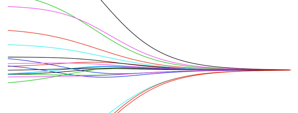
post_means <-
  QuickStartExample %>%
  rename(scale = y) %>%
  filter(x.1 > 100)
for (i in 1:100){
  laplace_scale <- seq(0.1, 0.001, length.out = 100)[i]

  blm_laplace <- stan_glm(y ~ ., data = QuickStartExample, seed = 1,
                          prior = laplace(location = 0, scale = laplace_scale),
                          iter = 1000,
                        refresh = 0)

  post_means <- rbind(post_means, c(coef(blm_laplace)[-1], laplace_scale))
}


library(reshape2)
names(post_means) <- c(names(QuickStartExample)[-21], "scale")
post_means %>%
  melt(id.vars = "scale") %>%
  mutate(scale_inv = 1/scale) %>%
  ggplot(aes(x = scale_inv, y = value, col = variable)) +
  scale_x_continuous(trans='log10') +
  geom_line() +
  theme_bw()